Fit Peaks/Autoindexing in GSAS-II
In this exercise you will use GSAS-II to search for a unit cell that matches a set of diffraction peaks -- a process known as auto-indexing. First peaks must be located and optimized and then indexing can be done.
1st Example: Fit Peaks/Autoindexing in GSAS-II
If you have not done so already, start GSAS-II.
Step 1: Read in the data file
1. Use
the Import/Powder Data/from GSAS powder data file menu item
to read the data file into the current GSAS-II project. This read option is set
to read any of the powder data formats defined for GSAS (angles in centidegrees, TOF in µsec). Other submenu items will read
the cif
format or the xye
format (angles in degrees) used by Topas, etc. In those cases, you would change the file
directory to
data file menu item to read the data file into the current GSAS-II project.
Because you used the Help/Download tutorial menu entry to open this page and
downloaded the exercise files (recommended), then the FitPeaks/data/...
entry will bring you to the location where the files have been downloaded. (It
is also possible to download them manually from https://advancedphotonsource.github.io/GSAS-II-tutorials/FitPeaks/data/.
In this case you will need to navigate to the download location manually.)
For this tutorial you should see the data file in the file browser, but if
extensions on data files are not the expected ones, you may need to change the
file type to All files (*.*) to find
the desired file.
2. Select the 11bmb_3844.fxye data file in the first dialog and press Open. There will be a Dialog box asking Is this the file you want? Press Yes button to proceed.
3. The file 11bmb_3844.prm instrument parameter file is automatically selected; it was produced by 11BM-B instrument processing software when the corresponding fxye file was created from the 12 detector raw data. If absent or the name doesn’t match the data file name, a file dialog will appear for you to select the correct instrument parameter file.
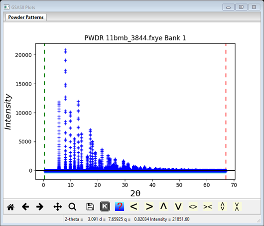
At this point the GSAS-II data tree window will have several entries

and the plot window will show the powder pattern
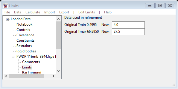
Step 2: Select Limits
This pattern has much more data than we need, so it is helpful to cut down the range. Click on the Limits item in the GSAS-II data tree. Use the New: row of entry boxes to set Tmin and Tmax to 4 and 27.5. Notice on the plot that the limit lines have moved to these positions; the green lower limit is just below the 1st peak and the red upper limit is in a wide gap between peaks. You may also drag the limit lines to the desired location or place them by a left mouse click on a data point for the lower limit or a right click on a data point for the upper limit.
Step 3: Determine Peak Positions
1. Click on the Peak List item in the GSAS-II data tree. This creates an empty window of peak positions (the Limits window is erased). At this point it is wise to zoom in on the data that will be used for indexing.
2. Click on the Zoom button (5th one from the left on the plot toolbar), then press the left mouse in one corner of the region to be used; holding the mouse button down, drag over the region to the opposite corner; a box will be drawn over the region to be zoomed and the plot will be redrawn with the new limits. The toolbar has a number of buttons to the right of the help button (‘?’) that can be used to incrementally change the view.
3. Important: Click on the Zoom button again to turn off the zoom mode.
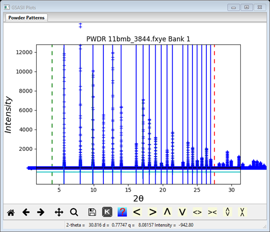
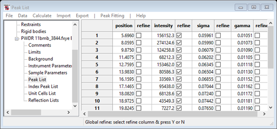
4. Under Peak Fitting in the menu select Auto search. The plot window will immediately show that all peaks were picked with a blue vertical line on each one

and peaks are shown in the Peak List window in order of increasing 2Q.

There will be 20 peaks in this example. You should examine both the list and the plot to be sure the auto search did not pick a peak twice (rarely) or skip a peak or shoulder. You can add a peak to the list by pressing the left mouse button with the pointer on a data point at the peak top or shoulder; be sure the zoom/shift buttons are off. You may drag a peak position as needed. A position may be deleted with a right click with the mouse on the blue line. You can also delete a peak by selecting the row in the table; it will be highlighted in blue. Then press the Delete key; it will be removed from the table and the plot. The list will always show the peaks sorted by position. When done you should have 20 unique peak positions.
Step 4: Refine Peak Positions
This refinement proceeds stepwise; first doing the default refinement and then adding parameters to complete the fitting,
1. Refine the peak intensities and the background. These parameters have their refinement flags turned on by default. Use the menu item Peak Fitting/Peakfit. Do NOT use the Calculate/Refine menu item; that should used for Rietveld/Pawley refinements. You will be asked to save the current project before the fit will proceed; change directory if desired and provide a suitable name (we assume LaB6). A window will show the progress of the refinement and will close when the least-squares fit is complete (usually very fast). The plot is updated with the fit, the peak list window is updated with the new peak values and a summary of the refinement is shown on the console window as well.
2. Now add refinement of the peak positions. This can be done by clicking on all the refinement flags for the individual peaks or it is possible to set them all at the same time using this recipe:
a. single-click on any value in the table to select it, for example the first peak position. A black box appears around the value.
b. single-click on the refine label above the peak position check-boxes. The entire column of checkboxes is highlighted in blue. Press the y key to turn on all refinement flags (n would turn them off).
Next, repeat the refinement using the Peak Fitting/Peakfit menu item.
Now, select peak widths for
refinement. This can be
performed in 2 different ways. Method 1: refine sigma (Gaussian
width) and/or gamma (Lorentzian width) for individual peaks. To do this,
click the refinement flags for sigma and/or gamma in the Peak List window.
Method 2: preferably, the LS refinement of peak
widths can be constrained to follow an instrumental broadening equation
as described below. Note - one cannot refine ALL peak widths using both
individual sigma & gamma values AND instrumental broadening
terms at the same time.
To constrain refined peak widths to an instrumental broadening equation, first select the Instrumental Parameters item in the data tree. This opens a window for peak profile terms and also creates a new plot window showing the instrument profile resolution curve.
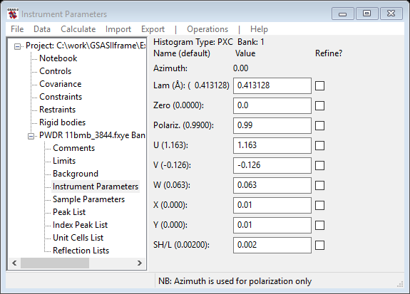
The plot window shows the resolution curves corresponding to the values of the Gaussian U, V, W, Lorentzian X & Y coefficients; ‘+’ marks show the individual values based on the sig & gam values for the peaks in Peak List. Select the refine flag checkbox for Gaussian U, V, W, and Lorentzian X, Y.
3. Then, repeat the refinement. First click on the Peak List item in the data tree and then refine using the Peak Fitting/Peakfit menu item. At this point a good fit should be seen by zooming in on individual peaks. For example see
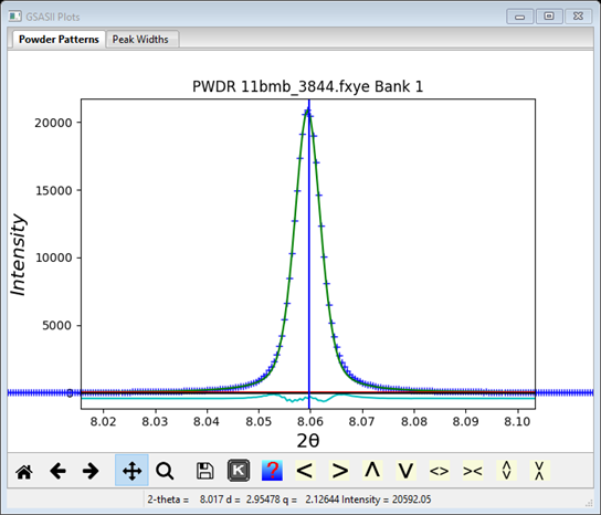
Notice that the peak position is slightly to the right of the peak top. This is a consequence of the peak asymmetry arising from axial divergence in the diffractometer. The Rwp is ~7% as shown on the console window. Again the Peak List entries are all updated with new values and those in Instrument Parameters are also updated.
Step 5. Prepare Indexing Peak List
A separate list of peaks is kept for use in autoindexing. It is found in the Index Peak List item in the data tree. In the initially empty window created by this action, use menu item Operations/Load/Reload to copy the fitted peaks from the Peak List.

Note that by default all peaks are selected to be used. You may choose to not use a fitted peak (e.g. if suspected it is from a contaminant).
Step 6. Run Autoindexing
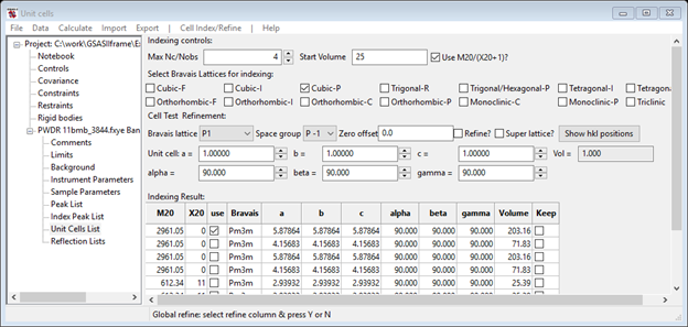
Select the Unit Cells List data item. This brings up a window for indexing and cell refinement options

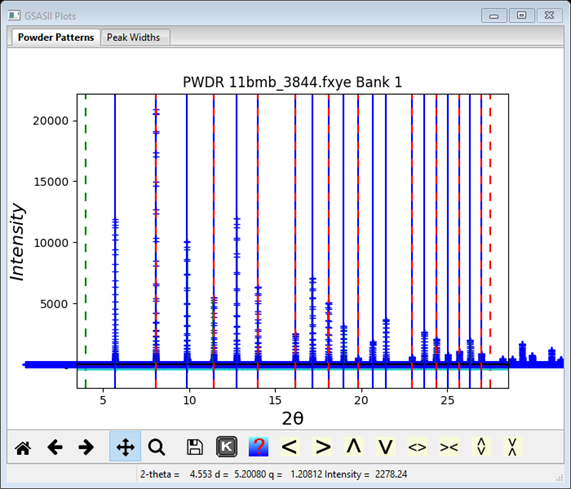
For the most rapid search (since we know the right answer), select Cubic-P and launch the search using menu item Cell Index/Refine/Index Cell. The search then runs and the console shows a running list of possible cells as they are found; the sorted by M20 list of possible matching cells is shown in the Unit Cells List window
Step 7. Review Cell Choices
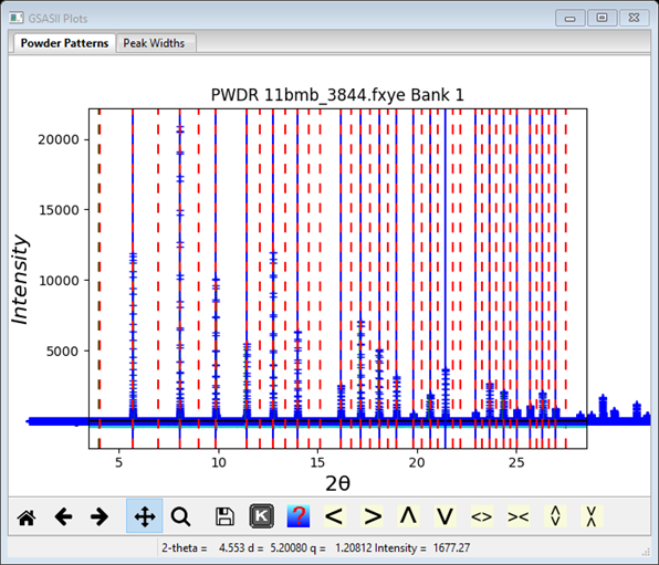
Review the list of cells associated with the Unit Cells List data item. Note that as one selects a unit cell, the generated reflections for that cell are shown in the plot with dashed red lines. Sliding the cursor over these lines shows a small popup window with the indexed hkl for them. Note how the first cell in the list (M20~2970) with a=5.87864 Å generates very many lines with no corresponding peaks (NB: this solution might not always show up!)
while the (M20~600) cell with a=2.93932 Å generates not enough lines to match all the peaks
Step 8. Select/Refine Cell
Select the cell with M20 ~ 2970 with a = 4.15683 Å. This indexes all peaks with almost a perfect fit to the peak positions (compare dashed red lines to solid blue ones). Import the cell information using the Cell Index/Refine/Copy Cell menu option. Then optimize the cell by refining the lattice parameters and the two-theta zero: click on the Refine? checkbox next to the Zero offset value and then the Cell Index/Refine/Refine Cell menu option. The M20 improves to ~3600 as the a cell parameter value shifts from 4.15683 to 4.15691 because the zero is now refined. (NB: The certificate value for NIST SRM 660a is 4.15692 Å). Press the Show hkl positions button to update the plot including the refined Zero offset (in this case hardly anything happens!).
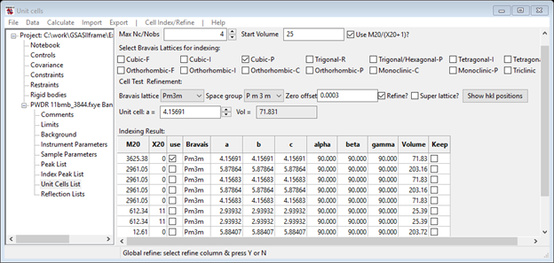
Notice that a new entry heads the list in the Indexing Result section of the Unit Cells List window with an improved M20(~3600) and a new value for Zero offset is shown. NB: the Show hkl positions button has an additional use; you can enter the Bravais lattice, Space group & Unit cell for any material. Then pressing Show hkl positions will use that cell to index the lines in Index Peak List. This might be useful to identify e.g. a second phase in your pattern.
(Optional) Finally, use of the Cell Index/Refine/Make new phase menu option allows one to create a phase with these lattice parameters in the data tree under Phases. A name for the new phase is requested. This creates the tree item Phases (if it wasn’t already present). This new phase can be used in future analysis (e.g. Rietveld or Pawley refinement).
To continue with the second part of this exercise, select the menu item File/New project in the GSAS-II data tree window. You will be asked if you want the current project saved; if Yes then all the peak fitting/indexing & cell refinement results will be saved to the LaB6.gpx file. If No then the file will remain as it was when created at Step 4 above.
2nd Example: Fit Peaks/Autoindexing in GSAS-II
In this exercise we will fit peaks and index them for the mineral jadarite (aka “kryptonite”). The data were also collected on 11BM-B at APS. The unit cell is monoclinic so it is a more substantial test of the indexing capability of GSAS-II. The required data files should have been downloaded when you downloaded this tutorial. Otherwise you will need to get them manually from https://advancedphotonsource.github.io/GSAS-II-tutorials/FitPeaks/data/. Be sure to get both 11bmb_6231.fxye and 11bmb_6231.prm
Step 1. Read in the data.
The file is FitPeaks\data\11bmb_6231.fxye; it has a corresponding prm file. Load them in & the plot is
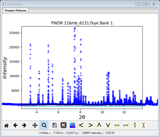
I’ve zoomed in & shifted the plot some to highlight the lower part of the pattern.
Step 2 Set limits
Set the limits as 3 and 9. This will give a suitable number of lines for indexing.
Step 3 Pick peaks
Pick all peaks you can see between the limits (including the small ones); use Auto search to start and then fill in by hand: Add peaks by left-clicking on a data point near the top of the peak. Peak positions can be moved by dragging the peak line and peaks can be deleted by right-clicking on them. This only works when the zoom and reposition modes (below) are not selected. Also note some peaks have shoulders most notably at 5.07, 6.04, 7.81deg. I found 28 peaks (there was one very weak shoulder at ~7.3 deg. I skipped – it might be from a second phase? We’ll see later).

Step 4. Refine peaks
Following the steps used in the LaB6 example above, refine the peaks and the profile shape parameters in Instrument Parameters. You will be asked for a project file name at the first refinement (I used ‘jadarite’). In the end my refinement converged at Rwp=11.41% and some peaks do show some discrepancy as the sample is more complex than the simple U, V, W, X, Y model can accommodate. Make sure no peaks drift away during refinement (one weak one at ~6.67 is particularly troublesome). However, this is good enough to proceed.
Step 5. Prepare Indexing Peak List
As before do Operations/Load/Reload in the Index Peak List window.
Step 6. Index the cell
Let’s assume that we know the cell is primitive monoclinic. In a real world case we wouldn’t know this and we would have to try each Bravais lattice. These can be done as a group, but it takes time to go through all the bad cases.
Select Monoclinic-P and do Cell Index/Refine/Index cell in the Unit Cells List window. Progress will be much slower and suitable results will be slow in coming so be patient. Watch the console window; the right answer will have an obviously large M20 (~380) and a volume of ~594Å3 (10th column of console display). Once this is seen (it may take more than one try to get this) you can stop the indexing search by pressing Cancel on the progress bar window. Notice the ‘keep’ column; this allows you to keep some solutions from one indexing run to the next. It may take more than one press to fully stop it. My result was

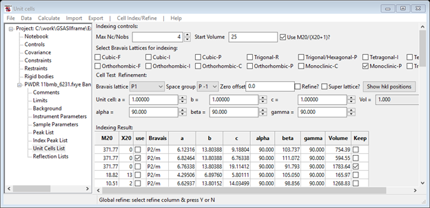
Notice there may be other equally good M20 results with different volumes; other solutions may be obtained as you keep trying the indexing. Be sure to use Keep to keep good ones as you try new indexing runs. The best solution is the one with the smaller volume and β > 90 deg. The plot shows every peak indexed including a weak peak not selected for the peak fitting, although the weak peak at 2Q~7.3 has a shoulder that wasn’t indexed. I presume that is a contaminant. Copy the best cell and try to refine it along with the Zero offset. I obtained an improved M20 ~444 and slightly different lattice parameters. Try different space groups, pressing the Show hkl positions each time to see which lines vanish. By sliding the cursor over the index lines without any visible peak you can see that the missing ones are 010, 100, 001, 110, 030, 111, 20-1, 10-2, 041, 050, 21-2 & 23-1. Many of these are accidental but the 0k0; k≠2n and h0l; h+l≠2n ones characterize the space group P21/n. Armed with this information you can Make new phase for the indexed cell (I called it ‘kryptonite’) and select Phases/kryptonite from the GSAS-II data tree.

Notice that the lattice parameters and space group have been set for you.
This concludes this exercise; do Save project as it is needed for the Charge Flipping in GSAS exercise. The features of the Phase Data window will be presented in other exercises.
3rd Example: Fit Peaks/Autoindexing in GSAS-II
In this exercise we will fit peaks and index them for sucrose in preparation for a charge flipping exercise. If continuing from the previous indexing example do File/New project from the main GSAS-II data tree menu; you will be asked if you wish to save the old project. The data were also collected on 11BM-B at APS. The unit cell is monoclinic so is another more substantial test of the indexing capability of GSAS-II. The required data files should have been downloaded when you downloaded this tutorial. Otherwise you will need to get them manually from https://advancedphotonsource.github.io/GSAS-II-tutorials/FitPeaks/data/. Be sure to get 11bmb_8714.fxye, 11bmb_8716.fxye and the corresponding .prm files.
Step 1. Read in the data.
The file is FitPeaks\data\11bmb_8716.fxye; it has a corresponding prm file and is for Domino® sugar ground under acetone. The other fxye file in this directory 11bmb_8714.fxye is for Domino® 10X powdered sugar used “as is” out of the box. Load the 8716 file in & the plot is
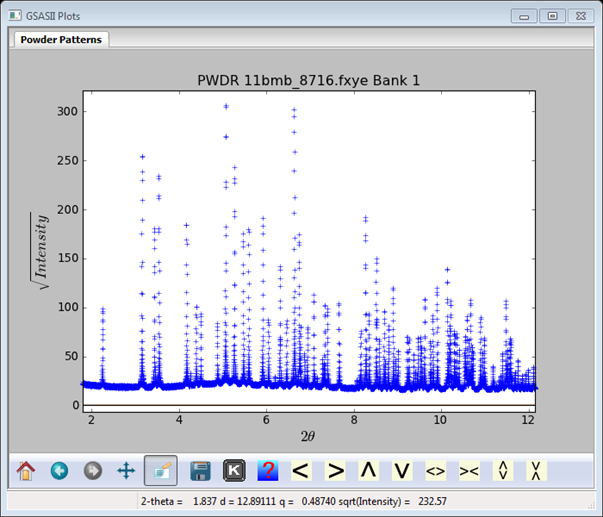
I’ve zoomed in & shifted the plot some to highlight the lower part of the pattern; I’ve also chosen to plot the square root of the intensity (use ‘S’ key) as this shows weak peaks better.
Step 2 Set limits
Set the limits as 2 and 8. Again, this gives a reasonable number of peaks for indexing.
Step 3 Pick peaks
Pick all peaks you can see between the limits (including the small ones); use Auto search to start and then fill in by hand: Add peaks by left-clicking on a data point near the top of the peak. Peak positions can be moved by dragging the peak line and peaks can be deleted by right-clicking on them. This only works when the zoom and reposition modes (below) are not selected. An easy to shift the view is to use the ‘<’ and ‘>’ buttons. Also note the shoulder at ~6.3 deg that should be added to the list. I skipped a couple of very weak peaks; the total list has >28 peaks.

Step 4. Refine peaks
Following the steps used in the LaB6 and kryptonite examples above, refine the peaks and the profile shape parameters in Instrument Parameters. You will be asked for a project file name at the first refinement (I used ‘sucrose’). In the end my refinement converged at Rwp=6.69% and some peaks do show some discrepancy as the sample is more complex than the simple U, V, W, X, Y model can accommodate. Make sure no peaks drift away during refinement. However, this is good enough to proceed.
Step 5. Prepare Indexing Peak List
As before do Operations/Load/Reload in the Index Peak List window.
Step 6. Index the cell
Let’s assume that we know the cell in primitive monoclinic. In a real world case we wouldn’t know this and we would have to try each Bravais lattice. These can be done as a group, but it takes time to go through all the bad cases.
Select Monoclinic-P and do Cell Index/Refine/Index cell in the Unit Cells List window. Progress will be much slower than for LaB6 but oddly much faster than for kryptonite and suitable results may appear almost immediately. Watch the console window; the right answer will have an obviously large M20 (~900) and a volume of ~704Å3 (10th column of console display). Once this is seen (it may take more than one try to get this) you can stop the indexing search by pressing Cancel on the progress bar window. Notice the ‘keep’ column; this allows you to keep some solutions from one indexing run to the next. It may take more than one press to fully stop it. My result was


Notice there may be other equally good M20 results with different volumes; still other solutions may be obtained as you keep trying the indexing. Be sure to use Keep to keep good ones as you try new indexing runs. The best solution is the one with the smaller volume and β > 90 deg and c>a (I got both solutions!). The plot shows every peak indexed including the weak peaks not selected for the peak fitting. Copy the best cell and try to refine it along with the Zero offset. I obtained an improved M20 ~1300 and slightly different lattice parameters. Try different space groups, pressing the Show hkl positions each time to see which lines vanish. The correct space group is P21. Armed with this information you can Make new phase for the indexed cell (I called it ‘sucrose) and select Phases/sucrose from the GSAS-II data tree.
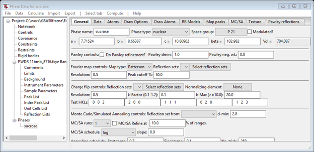
Notice that the lattice parameters and space group have been set for you. This concludes this exercise; Save the project file as it is needed for the sucrose Charge Flipping exercise. The features of the Phase Data window will be presented in other exercises.